


Having worked in manufacturing systems in Indonesia for a long time, I’ve noticed that compared to the past, customers frequently change order quantities and delivery dates. This makes it hard to revise production plans in time, affecting raw material procurement and often leading to discussions about having too much or too little inventory. Production Scheduler in Indonesia In Indonesia's Japanese manufacturing industry, the adoption of production management systems has been increasing. However, when it comes to one of the key challenges in production management—creating feasible production plans that take machine and equipment loads into account—manual work using Excel remains the standard practice. As a result, the demand for production schedulers is expected to grow in the future. 続きを見る
Generally, within the supply chain, too little inventory increases the risk of order backlogs and missed shipping opportunities, while too much inventory incurs interest costs—a classic trade-off problem.
To address this, I’ll explain how to build a system for demand forecasting that considers internal production equipment supply capacity, using case studies as examples.
The flow of this discussion will first outline the challenges faced by Indonesian manufacturing as issues of concern, clarify analytical perspectives as a framework for examining these issues, present system design methods as the main argument, and conclude with specific case studies.

Company Overview
Regarding our business, in addition to the production scheduler Asprova, we’ve developed a business development template called HanaFirst.
This is my personal opinion, but I believe only certain administrative tasks like accounting can be standardized. Operations like production management, inventory management, and order management are determined by relationships across the entire supply chain with customers and suppliers, making system standardization difficult.
Thus, while it’s labor-intensive, we must diligently gather business requirements and implement them into the system. HanaFirst’s concept is to shortcut this implementation process using templates.
Recent Challenges for Indonesian Manufacturing (Issues of Concern)
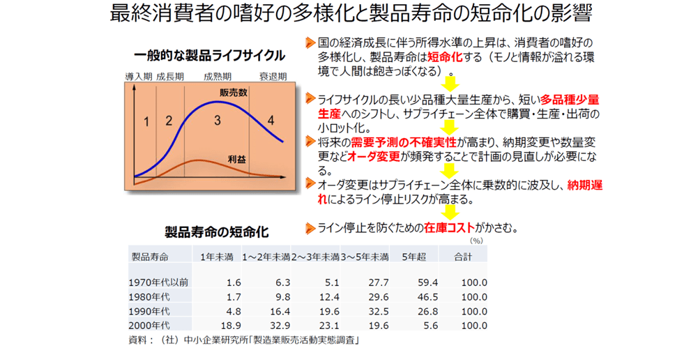
- As economic growth raises national income levels and information tools like SNS advance, final consumers’ preferences diversify. However, amidst a flood of goods and information, boredom sets in quickly, shortening product lifecycles.
- This makes demand forecasting within the supply chain harder. Combined with intensified competition from quality improvements by rival firms in other countries, order quantities inevitably shrink into smaller lots, and order changes become frequent.
- The burden of smaller lots and order changes has a multiplier effect across the supply chain, complicating optimal inventory control. To avoid opportunity loss, companies become conservative, leading to higher inventory costs.
 First, let’s confirm the challenges faced by Japanese manufacturing firms in Indonesia and clarify the issues of concern.
A typical product lifecycle follows the pattern of introduction, growth, maturity, and decline, as shown in the graph above. As a country’s economy grows and income levels rise, consumer preferences diversify and fragment, shortening product lifecycles.
This is evident in Japan: in an environment overflowing with goods and information, people grow bored quickly. Especially with the rise of SNS like Instagram and Facebook, new information spreads rapidly, and consumers shift to the next product just as fast.
In Indonesia, with a population of 260 million, 140 million are internet users—mostly via smartphones, primarily for SNS. This accelerates information diffusion and shortens trend cycles.
Essentially, there’s a shift from long-lifecycle, low-variety, high-volume production to short-lifecycle, high-variety, low-volume production, naturally increasing the trend toward smaller lot sizes in procurement, production, and shipping across the supply chain.
As product lifecycles shorten and customer order units shrink, companies’ procurement units to suppliers also shrink, leading to shorter lifecycles and smaller lots across the supply chain.
This automatically reduces the accuracy of future demand forecasts. Frequent order changes—delivery date or quantity adjustments against initial forecasts—necessitate plan revisions.
Order changes ripple multiplicatively across the supply chain, increasing the risk of production line stoppages due to delayed raw material deliveries from suppliers. To mitigate this, companies hold extra inventory, driving up costs in a vicious cycle.
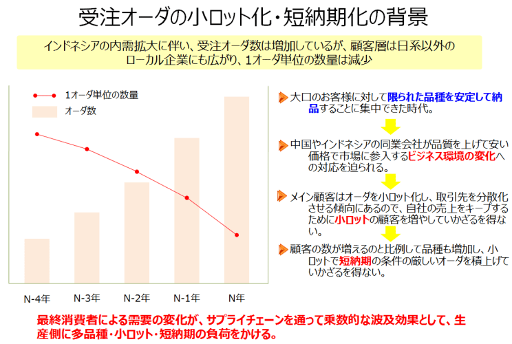
With Indonesia’s growing domestic demand, order numbers are rising, but the customer base now includes non-Japanese local firms, reducing per-order quantities.
Previously, the top priority was delivering to key customers on time without delays. Now, with smaller lot sizes flowing through the supply chain, customer numbers grow, and delivery destinations diversify.
As you know, manufacturers from China, Korea, and Hong Kong have entered Indonesia, and local manufacturers’ quality has improved. Companies can’t refuse small-lot, short-delivery orders.
Recently, an Indonesian official supporting SMEs noted that while 90% of cars on the road are Japanese, Japanese parts makers’ local procurement rates are extremely low. With 20,000 Japanese residents compared to 50,000 Koreans, they urged more Japanese presence.
Korea’s unemployment rate is about double Japan’s 2.5%, so many come with a do-or-die mindset, unlike Japanese expatriates assured of returning home after a five-year term. This suggests an increasingly tough business environment for Japanese firms.
Alongside these changes, shifts in final consumer demand impose a multiplier effect through the supply chain, burdening production with high-variety, small-lot, short-delivery demands.
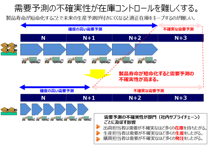
As mentioned, shorter product lifecycles make future production forecasts harder, complicating optimal inventory maintenance.
When maintaining optimal inventory becomes difficult, department heads in the internal supply chain grow conservative, fearing shipping, production, or supply delays. Shipping staff want more inventory as demand uncertainty rises, production staff want to produce more, and procurement staff want to order more.
Late raw material deliveries from suppliers halt production lines—a scenario to avoid at all costs. However, delays occur due to supplier constraints or unreasonable order conditions from our side.
Supplier procurement delays or equipment issues causing late deliveries are beyond control, but the complexity of procurement due to smaller lot sizes in the supply chain—leading to無理な schedules or delivery changes requested from suppliers—is a self-inflicted issue.
Raw material delays require production plan revisions, reducing productivity with line stoppages, increasing fixed costs via overtime or weekend work for recovery, and worsening company profitability.
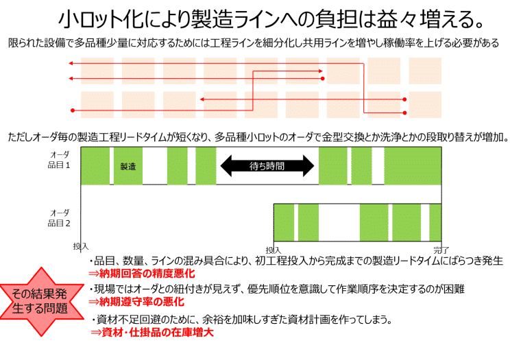
To handle high-variety, low-volume production with limited equipment, process lines must be subdivided, shared lines increased, and utilization rates boosted. However, per-order production lead times shorten, and with high-variety, small-lot orders, setup changes like mold swaps or cleaning rise.
This causes variability in production lead times from initial input to completion—due to item type, quantity, and line congestion—reducing delivery date accuracy. On-site, linking orders becomes unclear, making it hard to prioritize tasks, worsening on-time delivery rates.
To avoid material shortages, overly conservative material plans increase material and work-in-progress inventory.
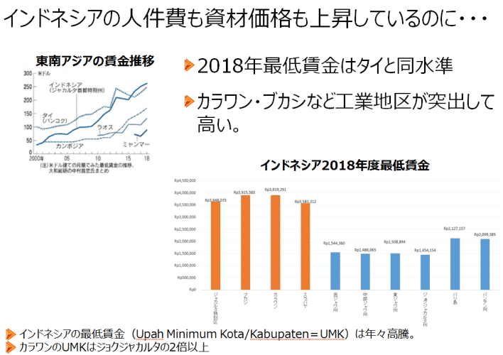
While not directly tied to supply chain material flows or factory production, one serious issue for Japanese firms in Indonesia is the annual rise in minimum wages.
In the West Java industrial belt (Jakarta, Bekasi, Karawang), wages are about double those in Central Java, explaining the appeal of migrant work.
Indonesia is often said to strongly protect workers’ rights. Under Labor Law (UU No 13 Tahun 2003), the trickiest part is termination payments: severance (uang pesangon), service recognition pay (uang penghargaan masa kerja), and compensation for lost entitlements (uang penggantian hak yang seharusnya diterima). Like a supersized ramen order, termination costs pile up significantly.
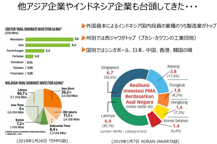
Among foreign firms in Indonesia, manufacturing leads by industry, with West Java (Bekasi, Karawang industrial parks) hosting the most, followed by Singapore, Japan, China, Hong Kong, and Korea by country.
As noted, many from China and Korea come with a high-stakes mindset, unlike Japanese staff guaranteed repatriation after five years. This reflects Indonesia’s increasingly tough business climate.
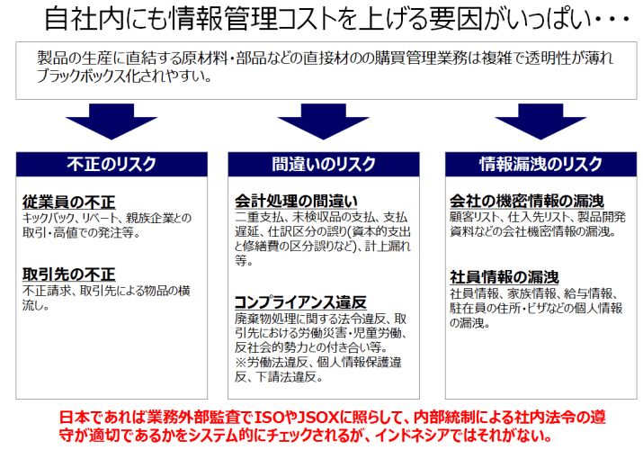
In Japan, JSOX (internal control rules under the 2006 Financial Instruments and Exchange Act) emphasizes IT controls and audits for corporate compliance. In Indonesia, it’s a sieve-like state.
Demand Forecasting and Inventory Costs in the Supply Chain (Analytical Perspective)
- Supply Chain Management involves managing the company as the center between upstream raw material suppliers and downstream final consumers. Goods flow with added value, but changes in demand and supply ripple outward with amplifying effects.
- Synchronizing and centralizing planning across departments improves demand forecast accuracy, shortens internal inventory retention, prevents opportunity loss, and achieves optimal inventory to reduce costs.
- Inventory costs consist of manufacturing costs and SG&A, but there’s also an invisible financial inventory interest cost, an off-balance-sheet liability that later manifests as profit compression.
- Reasons for bearing inventory costs in-house include bridging production and order lead time gaps and maintaining buffers to avoid stopping bottleneck processes.
- To maintain optimal inventory, PO issuance and production instructions within the internal supply chain must rely on accurate demand forecasts.
- If demand forecasts were 100% accurate or supply capacity were 100%, zero inventory would suffice. In reality, limited supply capacity requires minimal safety stock while aligning demand, adjusting business, sales, production, and procurement plans for the shortest linkage—today’s theme, impossible without considering supply capacity in forecasts.
- Thus, supply chain capability is measured by responsiveness, flexibility, and reliability.
Next, I’ll outline analytical perspectives to address recent Indonesian challenges—burden from high-variety, low-volume production, increased planning revision load from frequent order changes, and difficulty in optimal inventory control—raised in the previous section.
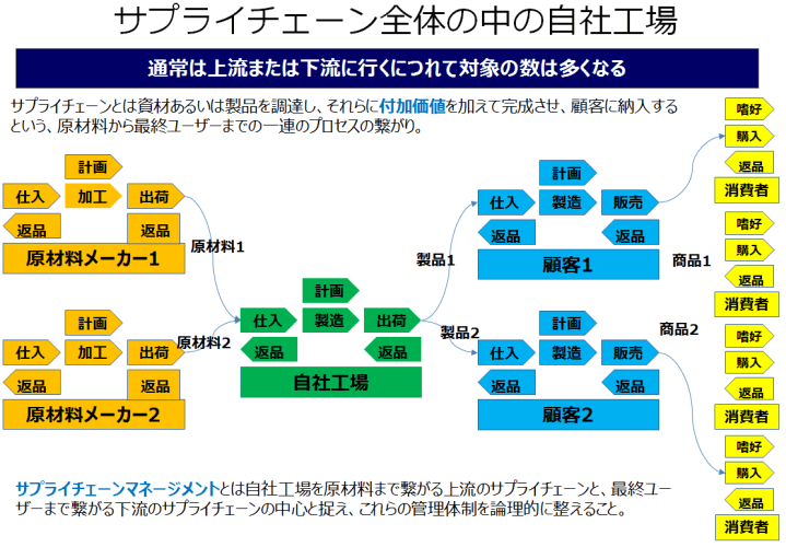
This diagram shows “our factory’s position in the supply chain.” Typically, the number of players increases upstream or downstream from the factory.
The supply chain is a series of processes from procuring materials or products, adding value, and delivering to customers—from raw materials to end users. Supply Chain Management involves logically organizing this, viewing the factory as the center of upstream (to raw materials) and downstream (to end users) chains.
Today, various business models exist, and shady online schemes abound, with many fixated on extracting money digitally. Fundamentally, economic activity involves goods and services flowing through the supply chain with added value.
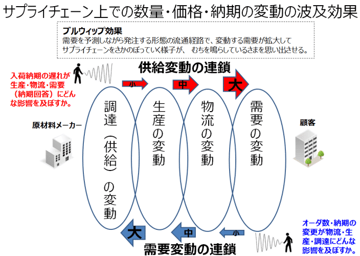
Supply fluctuations from upstream to downstream and demand fluctuations from downstream to upstream amplify as they chain through the supply chain, a whip-like motion called the bullwhip effect.
Specifically, raw material supplier delays amplify impacts on production, logistics (shipping), and final consumers, while consumer demand changes amplify effects on logistics, producers, and raw material suppliers.
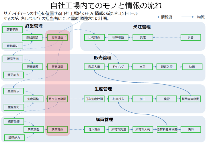
Controlling the flow of goods and information within our factory, at the supply chain’s center, relies on plans adjusted for supply and demand by each department’s staff.
While plans are made at each level based on supply-demand adjustments, they’re typically created independently without coordination. This may optimize individual departments but not the company as a whole—a phenomenon called partial optimization.
As mentioned, economic activity involves goods and services flowing with added value. When departments create partially optimized plans, connections between them become disjointed, likely causing unnecessary inventory buildup and failing to achieve optimal inventory.
So far, we’ve focused on material flows. Now, let’s consider costs incurred by goods flowing through the supply chain.
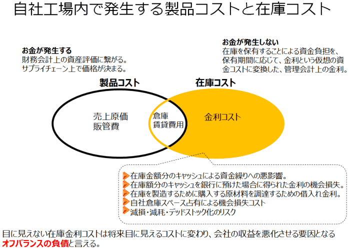
Manufacturing products incurs direct material costs, direct labor costs, and manufacturing overheads—collectively manufacturing costs—followed by SG&A costs like storage and advertising.
These are recorded as expenses in financial accounting, but holding inventory imposes a cash burden without direct outflow, converted into a managerial accounting inventory interest cost based on retention period.
Inventory interest costs include cash flow strain from inventory value, lost interest from banking that cash, borrowing costs for raw material purchases, opportunity costs from warehouse space occupation, and risks of impairment, spoilage, or dead stock. These invisible costs, unrecorded in accounting entries, later become visible, harming profitability as off-balance-sheet liabilities.
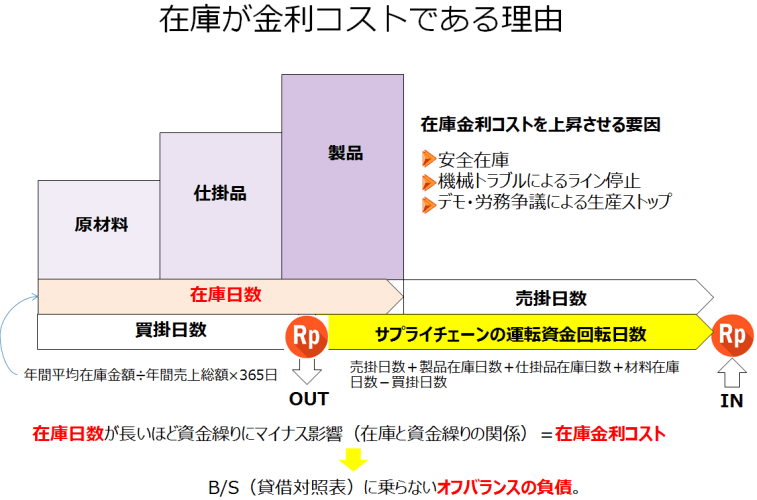
Factors raising inventory interest costs include safety stock, line stoppages from machine issues, and production halts from protests or labor disputes. Longer inventory days negatively impact cash flow, making it an off-balance-sheet liability not reflected on the B/S.
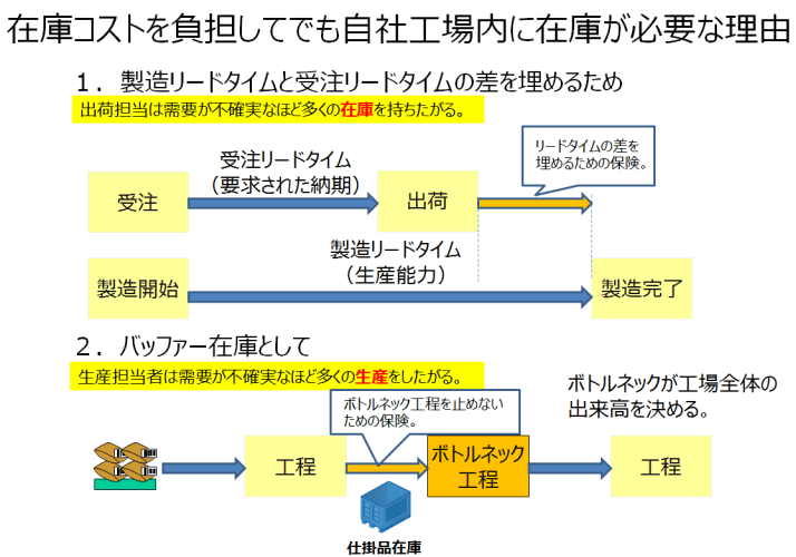
This might paint inventory as a villain, but there are legitimate reasons to bear its costs in-house.
One reason is to bridge the gap between production and order lead times. Typically, the order lead time from customer order to shipment is shorter than the production lead time from start to finish, requiring inventory as insurance for the difference.
Another is the need for buffer inventory to keep bottleneck processes—determining factory productivity—running.
Shipping staff want more inventory as demand uncertainty grows, and production staff want to produce more to avoid opportunity loss—a psychological drive.
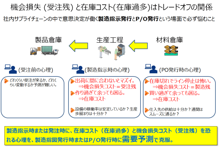
In manufacturing operations, two key supply chain quantity decisions occur: PO issuance and production instruction issuance. The “trade-off between opportunity loss (order backlog) and inventory costs (excess inventory)” means: at PO issuance, stockouts halting lines are feared, but overbuying is troublesome; at production instruction issuance, missing shipment deadlines is bad, but overproducing is problematic.
Thus, maintaining optimal inventory requires overcoming fears of inventory costs (excess) and opportunity loss (backlogs) with accurate demand forecasts at PO or production instruction issuance.
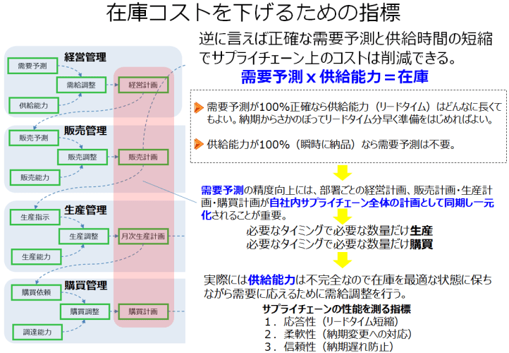
In extremes, if demand forecasts were 100% accurate, preparing lead time ahead of due dates would suffice regardless of supply capacity (lead time). If supply capacity were 100% (instant delivery), forecasts wouldn’t be needed—both achieving zero inventory.
In reality, supply capacity constraints necessitate minimal safety stock while meeting demand, adjusting business, sales, production, and procurement plans for the shortest linkage.
Thus, supply chain capability metrics are responsiveness (lead time), flexibility (change adaptation), and reliability (on-time delivery).
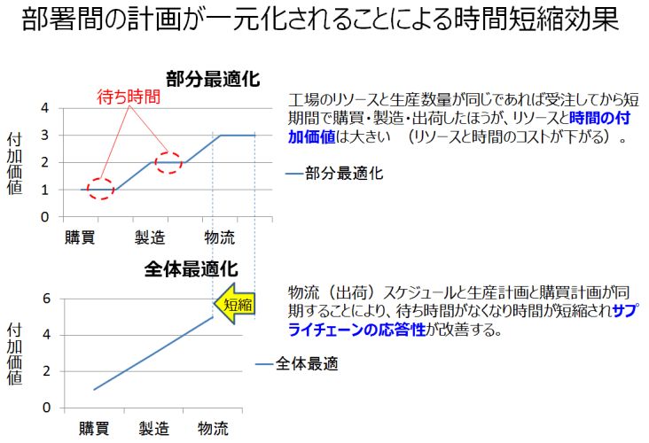
Department-specific supply-demand plans—business, sales, production, procurement—optimized for each aren’t necessarily optimal for preceding or following departments, causing wait times.
Overall optimization means seamlessly linking department plans.
Systemizing Planning with Supply Capacity Consideration (Main Argument)
-
- Planning production with departmental supply capacities means creating an overall optimized plan where business, sales, production, and procurement plans connect without strain.
- In systemizing planning, differing inter-process supply capacities mean varying takt times, making the slowest bottleneck process the factory’s production capacity.
- After lead time offsetting, overloaded tasks on specific days are shifted to other days or equipment—APS automates this.
- Fixed lead time plans, ignoring process capacity, are rough, while cycle-time-based plans consider capacity for a seamlessly connected, overall optimized plan.
- MRP’s infinite capacity loading with fixed lead time offsetting is a capacity plan; MRPII’s finite capacity leveling with cycle times is a cycle-time plan.
So far, we’ve seen that recent challenges for Japanese manufacturers in Indonesia—burden from high-variety, low-volume production, planning revision load from frequent order changes, and optimal inventory control difficulty—stem from a trade-off between opportunity loss risk and inventory interest costs in supplier-customer supply chain dynamics. Addressing this requires demand forecasting with production equipment supply capacity in mind. Here, we’ll explore designing such a system.
“Supply capacity varies” means takt and lot sizes differ between upstream (molding, pressing) and downstream (assembly, welding) processes, often leading to intermediate inventory buildup upstream for downstream digestion. Reducing setup time requires larger lots, while reducing inventory needs smaller lots—overall optimization considers inter-process capacity and setup times.
Lot sizes flowing between processes depend on the bottleneck, whose delayed takt affects overall takt and output.
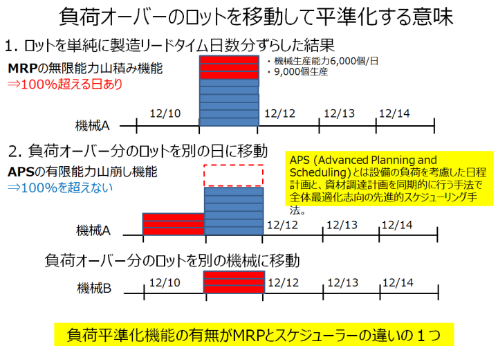
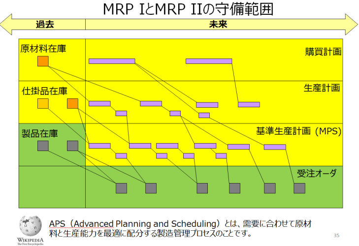
When planning production, lead times are offset by day, but simply offsetting can overload specific days beyond equipment capacity—commonly called MRP (Material Requirement Planning) lead time offsetting.
Overloaded tasks must shift to other days or equipment. APS (Advanced Planning and Scheduling), or “先進的計画&スケジューリング” in Japanese, is an overall optimization-oriented advanced scheduling method considering equipment load. The production scheduler Asprova, introduced today, realizes APS in a system.
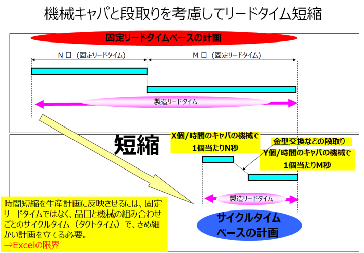
To “shorten lead time with machine capacity and setup consideration,” set cycle times (seconds per unit for specific equipment) instead of fixed lead times.
Fixed lead time plans, ignoring process capacity, are rough, while cycle-time-based plans consider capacity for a seamlessly connected, overall optimized plan.
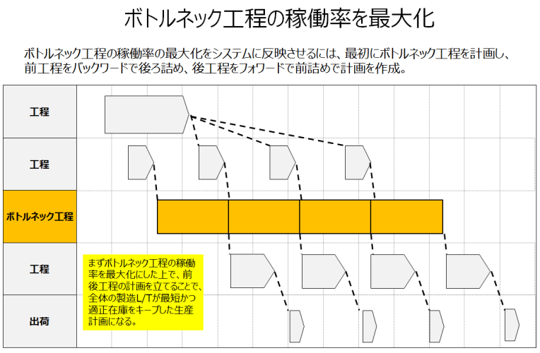
As noted, supply capacity varies, and factory production capacity hinges on the bottleneck. Planning maximizes bottleneck utilization, then schedules preceding and following processes for overall optimization.
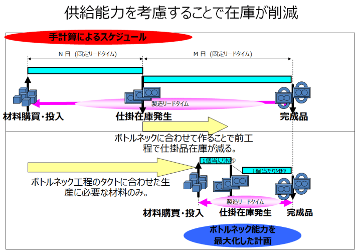
Centering plans on the bottleneck eliminates work-in-progress buildup before it, ensuring just-in-time flow of necessary items aligned with bottleneck takt.
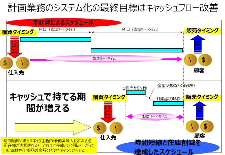
Considering supply capacity seamlessly connects processes, shortening production lead times and reducing in-process inventory, lowering inventory interest costs, extending cash retention, and boosting profitability.
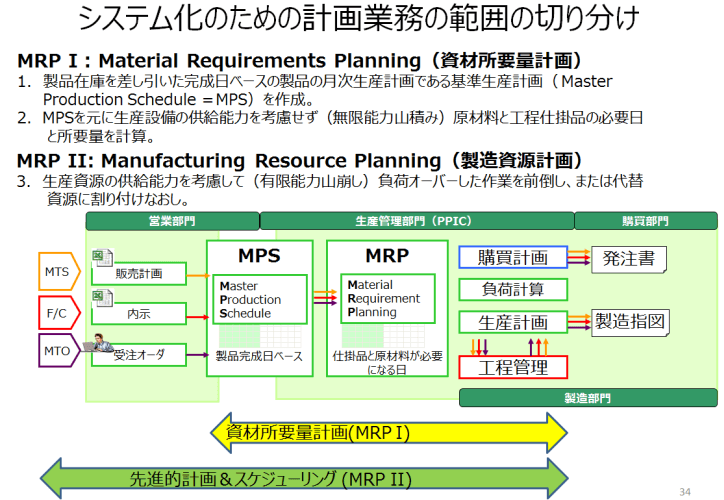
Expressing this systematically: MRP’s infinite capacity loading with fixed lead time offsetting is a capacity plan; MRPII’s finite capacity leveling with cycle times is a cycle-time plan, corresponding to APS.
End-to-End System Case Study from Order to Procurement (Conclusion: Examples)
- So far, we’ve discussed how planning with cycle times (seconds per unit) to maximize bottleneck utilization shortens lead times, reduces inventory, and improves cash flow by considering supply capacity. Now, we’ll explore systemizing this flow.
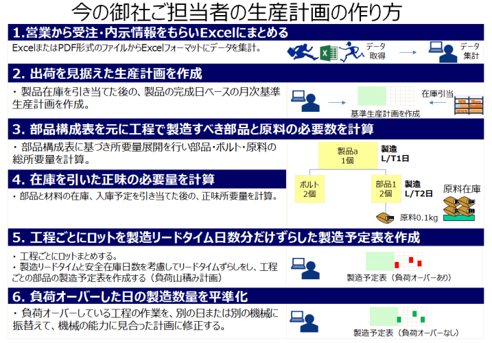
- Current production planning starts with order data to create a shipping plan, followed by a monthly production plan based on product completion dates. MRP calculates requirements via the BOM, offsets net requirements (post-inventory deduction) by lead time for a production schedule, and levels overloaded tasks by shifting days or equipment.
- In this manual planning, poor sales-production communication often leads to production-centric plans, and even leveled plans remain partially optimized with excessive wait times.
- For overall optimization, end-to-end management from order to production and procurement is needed to create production flow.
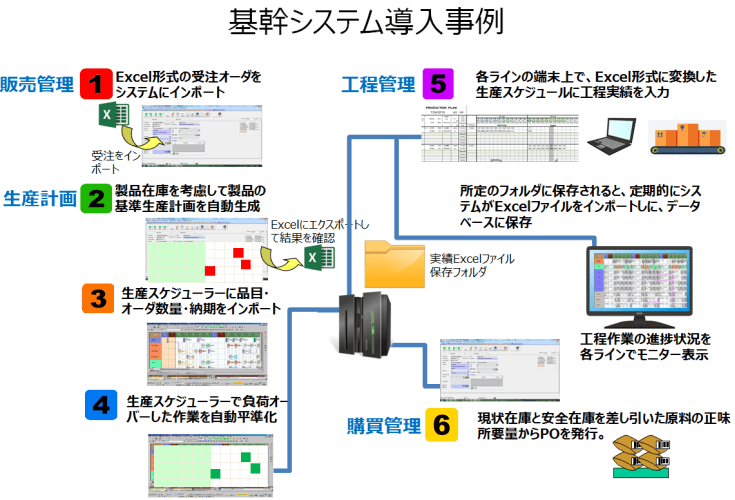
Summarizing prior sections, I’ll present a system implementation example achieving lead time reduction, inventory reduction, and cash flow improvement via cycle-time-based, finite-capacity load leveling.
Sales gathers order/forecast data in Excel, creates a production plan for shipping, calculates required parts and materials per process via the BOM, computes net requirements after inventory deduction, offsets production lots by lead time days per process, and levels overloaded days’ quantities.
Leveling overloaded days—shifting tasks to other days or equipment—creates a chain reaction of displacing pre-assigned tasks, making adjustments challenging.

First, sales plans shipments to meet customer needs, but PPIC staff, focusing solely on production, create discretionary plans, leading to partial optimization. This delays status updates and delivery responses to customers, as well as handling order quantity/delivery changes and rush orders.
Second, Excel-based planning inevitably optimizes lots for each process without considering preceding/following process capacities or loads. Simple lead time offsetting followed by leveling tends toward partial optimization, potentially overwhelming downstream processes, increasing wait times and inventory.
To avoid partial optimization and create an overall optimized plan, end-to-end management from order to production and procurement is essential for production flow.
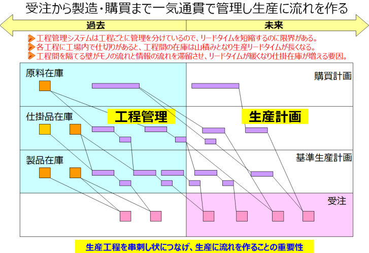
Process management systems, dividing control by process, limit lead time reduction. Internal process barriers stack inventory between processes, lengthening production lead times. These barriers stagnate material and information flows, easing lead times and increasing work-in-progress.
This underscores the importance of串刺し (skewering) processes to create production flow.
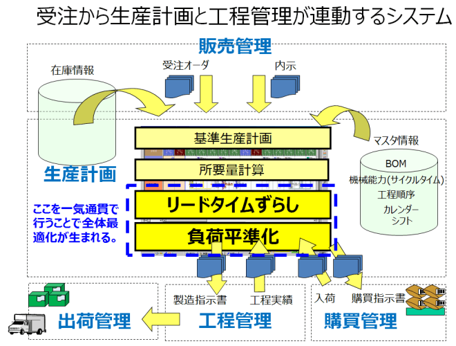
Seamless linkage from order data to production planning, procurement orders, process performance management, and shipping is critical.
This is the system implementation image of the “system linking orders, production plans, and process management” overview.
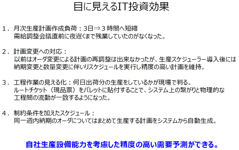
Post-system “visible IT investment benefits” include:
-
- Monthly production plan creation load: Reduced from 3 days to 3 hours—no more late-night overtime before supply-demand meetings.
- Handling plan changes: Previously, order changes couldn’t be re-adjusted, but post-scheduler, rescheduling for delivery/quantity changes maintains high-accuracy plans.
- Process task visibility: Site staff know which days’ shipments are being produced. Attaching route tickets to pallets aligns system links with physical inter-process flow.
- Constraint-based scheduling: Orders due within the same week are automatically consolidated into production plans.
Orders due within the same week are automatically consolidated into production plans.
Enables highly accurate demand forecasting considering internal production equipment capacity.
Functions of Production Scheduler Asprova
For basic function details, refer to the December 2018 seminar.
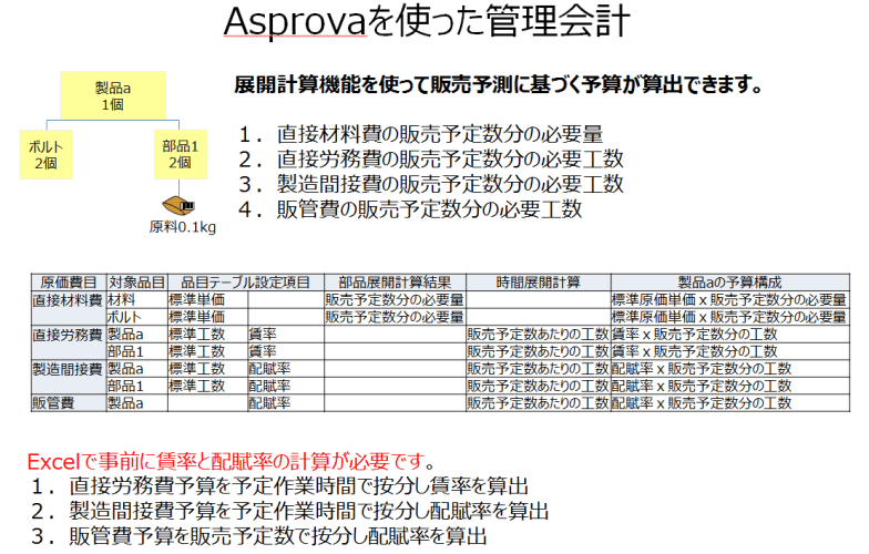
In Asprova’s item table, set material standard unit prices, labor rates (cost per minute) and efficiency (minutes per unit) or utilization (cost per minute) or allocation rates (cost per unit) for work-in-progress and products, calculate standard unit prices, and derive cost budgets based on sales forecasts to aid pricing decisions:
- Direct material costs: Standard unit price × planned input quantity
- Direct labor costs: Labor rate × efficiency × planned production quantity
- Depreciation costs: Utilization rate × efficiency × planned production quantity
- Other expenses: Allocation rate × planned production quantity
Using next period’s sales forecast, Asprova’s MRP calculates planned production quantities and direct labor hours for products/work-in-progress, and planned material input quantities.
However, Asprova doesn’t auto-calculate labor or allocation rates from budgets, so these are computed in Excel externally and set in the item table.
This enables cost budgets and per-unit standard prices based on next period’s sales forecast, facilitating pricing simulations.
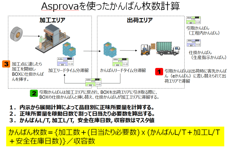
In Indonesia, firms supplying four-wheeler parts to TMMIN (PT Toyota Motor Manufacturing Indonesia) or ADM (PT Astra Daihatsu Motor) likely have production lines where goods flow per kanban.
Import next month’s forecast into Asprova, calculate net requirements per item via MRP, divide by operating days for daily needs, and compute kanban cards using kanban L/T, processing L/T, safety stock days, and capacity from the master, adjusting monthly circulating kanban cards.