Difference Between Infinite Capacity Loading and Finite Capacity Leveling in a Production Scheduler

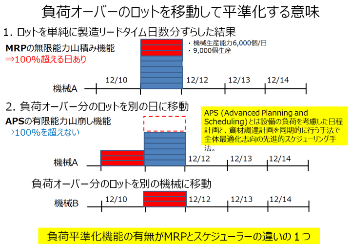
Typically, MRP is referred to as infinite capacity loading, which checks whether orders fall within production capacity. In contrast, the finite capacity leveling of a production scheduler verifies whether a feasible schedule can be created without delays in delivery.

Differences in Quantity-Based and Time-Based Production Scheduling Perspectives That Often Pose Challenges in Indonesia

Based on my experience, most manufacturing sites in Indonesia create production plans with a quantity-based mindset, focusing on how many units can be produced per shift or per day against the capacity of machines or lines.
If production plans have been created for years using Excel cells representing one shift or one day, it’s only natural that this mindset becomes the norm.
On the other hand, a production scheduler operates with a time-based mindset, assigning operations to available time slots, such as from 8:00 to 17:00.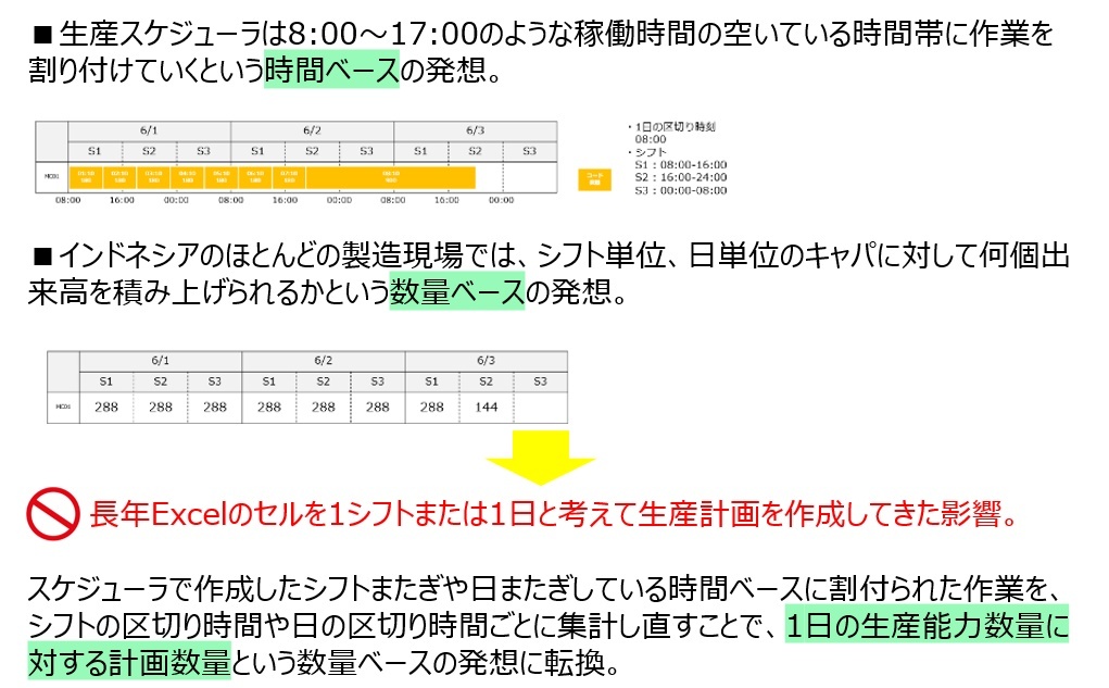
In IT terms, the difference can be expressed as whether objects are generated per shift or day or per manufacturing instruction. Although both approaches aim to create a production plan, I feel this conceptual gap is not easily bridged.
Therefore, when implementing a production scheduler in Indonesia (and likely across Asia), operations assigned on a time basis—spanning shifts or days—need to be re-aggregated based on shift or daily cutoff times.
It’s unclear whether Excel as a tool aligned with human logic or if human thinking has been overly influenced by Excel’s characteristics. However, it seems certain that unless the system makes an effort to adapt to this reality, it won’t be accepted by manufacturing site personnel.

Role of the Production Management Department

Relationship Between Production Planning and Capacity Planning

In Indonesia, as in Japan, the production management department (PPIC = Production Planning Inventory Control) in manufacturing creates a daily-adjusted Master Production Schedule (MPS) based on confirmed customer orders or forecast information, taking product inventory and manual adjustments into account.
This MPS is exploded into material requirements according to the Bill of Materials (BOM), and production orders are created considering lead times. However, in Indonesia, it’s rare to use an MRP (Material Requirement Planning) module in a production management system to generate production orders; typically, this is done in Excel.
By arranging these production orders chronologically, a monthly production schedule per item is created—this is what’s commonly referred to as Production Planning.
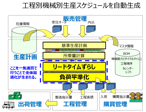When formulating a production plan and issuing manufacturing instructions to the shop floor, assignment to production lines is required. The workload on the lines at this stage is called Loading. Capacity Planning involves predicting whether existing resources can handle this load, and during production preparation, it may involve redistributing the load, adding overtime, or increasing lines.
Thus, production planning and capacity planning are inseparable, and errors in capacity planning directly lead to errors in production planning (delivery delays).

Planning Tasks of the Production Management Department

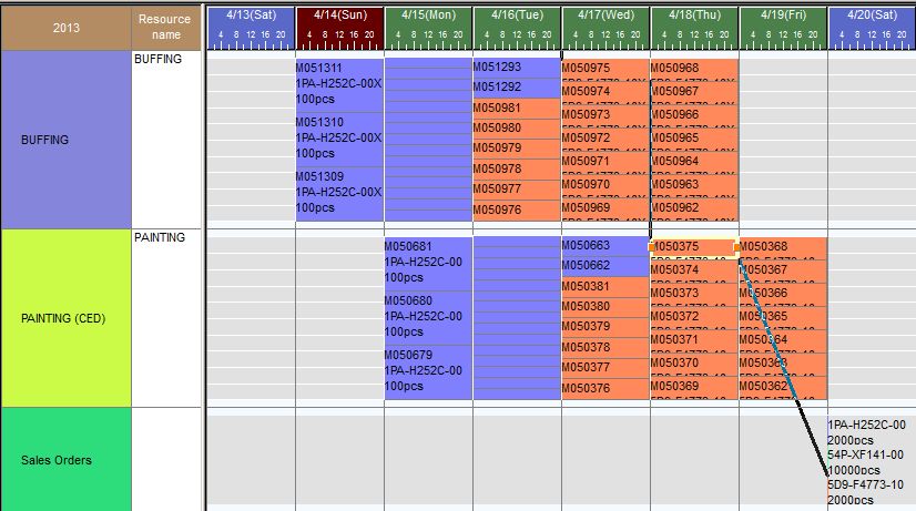
The MRP in a production management system is an infinite capacity backward plan that does not consider capacity planning. It tentatively stacks production orders by line, manually leveling them to alternative resources or schedules while confirming the availability of production resources and operating time to process the orders.

In MRP, inter-process operations are vertically linked

In contrast, a finite capacity leveling production plan, which considers capacity, allows you to see how much overflow occurs within the constraints of current resource availability and operating time.

Difference Between Forcing Assignment of Overflow Operations vs. Ignoring Them

Forced Assignment vs. Ignoring

If the planning parameters include an adjustment command, you can control how overflows (when time constraints are violated or the planning period is exceeded) are assigned. Without an adjustment command, these parameters are ignored.
Forced assignment means cramming operations into the period with infinite capacity, while ignoring means assigning with finite capacity within the period and infinite capacity outside it, without further consideration.

Assignment Behavior in Backward Scheduling

In backward scheduling, if nothing is set for "When exceeding the assignment start date/time," it behaves like forced assignment (infinite capacity), stacking operations to the right of the planning base date (within the planning period). This is because planning for the past is meaningless.
To stack overflow operations in backward scheduling to the left of the planning base date (outside the planning period), set "When exceeding the assignment start date/time" to "Ignore" (allowing penetration with infinite capacity assignment).

Assignment Behavior in Forward Scheduling

In forward scheduling, if nothing is set for "When exceeding the assignment end date/time," it behaves like ignoring (penetration with infinite capacity assignment), stacking operations to the right of the assignment end date/time (outside the planning period).
To stack operations within the planning period in forward scheduling, set "When exceeding the assignment end date/time" to "Forced Assignment" (infinite capacity assignment).

Checking Load Status for a Production Plan Without Delivery Delays

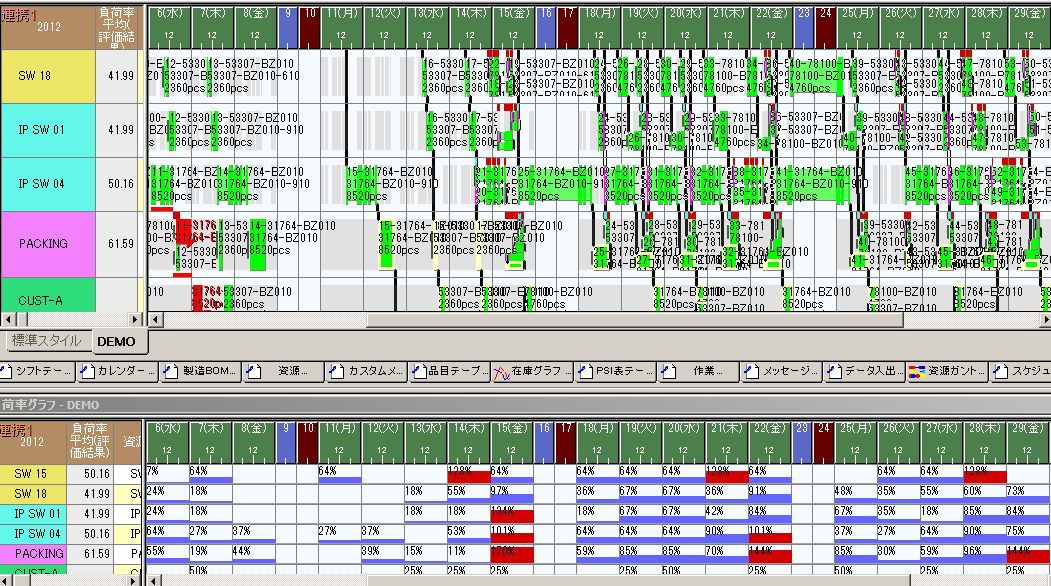
Production planners naturally aim to create plans without delivery delays. However, equipment capacity isn’t always sufficient, so they check daily load levels and where overloads occur, taking preemptive measures.
By assigning forward and enforcing forced assignment (infinite capacity) only when time constraint violations occur (exceeding the latest end date/time or earliest start date/time), planners can identify resources and periods with overloads (capacity shortages).
Notably, backward scheduling inherently considers due dates, so delivery delays don’t occur—only overloads do.

The earliest start date/time and latest end date/time serve as criteria for time constraint violations. In forward scheduling, exceeding the latest end date/time (or the earliest start date/time of a subsequent process) means "the preceding process is too late, and the subsequent process can’t be completed on time."
Based on this, planners decide, "At this point, there’s X% overload, so we’ll adjust the production plan or add overtime."

Cycle Time Plan vs. Capacity Plan

Leveling operations stacked based on cycle time aims to sequence operations, balance loads, and create a theoretically feasible plan without time constraint violations, emphasizing the calendar (horizontal axis) in an operation scheduling plan.
However, even if operations are sequenced and instructions are issued to the shop floor, it’s often difficult to execute them in that exact order due to on-site circumstances. Reflecting constantly changing factors affecting the plan into the system for rescheduling may not be practical.
If so, under the condition of avoiding delivery delays, it’s more realistic to stack operation lots within the daily capacity (production quantity or operating time) and issue instructions like, "Please process this many operation lots on each line today." This method prioritizes resource capacity (vertical axis).

For "1 lot per day: daily capacity 8,000 units, 5 machines, resource quantity 40,000 units":

For "1 lot per hour: daily capacity 8,000 units, 1 lot 1,000 units, 1 machine, resource quantity 8,000 units":

Checking Load with "Stacking" and Verifying Feasibility with "Leveling"

MRP’s load calculation function sets standard loads (cycle times) per item and line, calculates the minutes of load per line based on order quantities, shifts them by lead time (days), and stacks them against daily line capacity to determine daily wins or losses.
To determine whether the overflow of line capacity identified from daily "stacking" can meet due dates by advancing (assigning earlier), "leveling" is performed. A production scheduler automates this process.

"Leveling" means sequencing operations to avoid time constraint violations and creating a "theoretically feasible" schedule, emphasizing the calendar (horizontal axis) in an operation scheduling plan.
However, it’s impossible for humans to set all shop floor constraints 100% accurately in the scheduler for an optimized schedule. Thus, rather than idealistically applying the "leveling" result directly as the shop floor schedule, confirming that "leveling" roughly avoids delivery delays is sufficient. A practical system operation then involves setting safety stock for a few days as a buffer.
Under the condition of avoiding delivery delays, listing operation lots within daily capacity and issuing instructions like, "Please process this many operation lots on each line today," is more realistic, prioritizing resource capacity (vertical axis).

Relationship Between Inter-Process Overlap, Safety Stock, and Lot Size

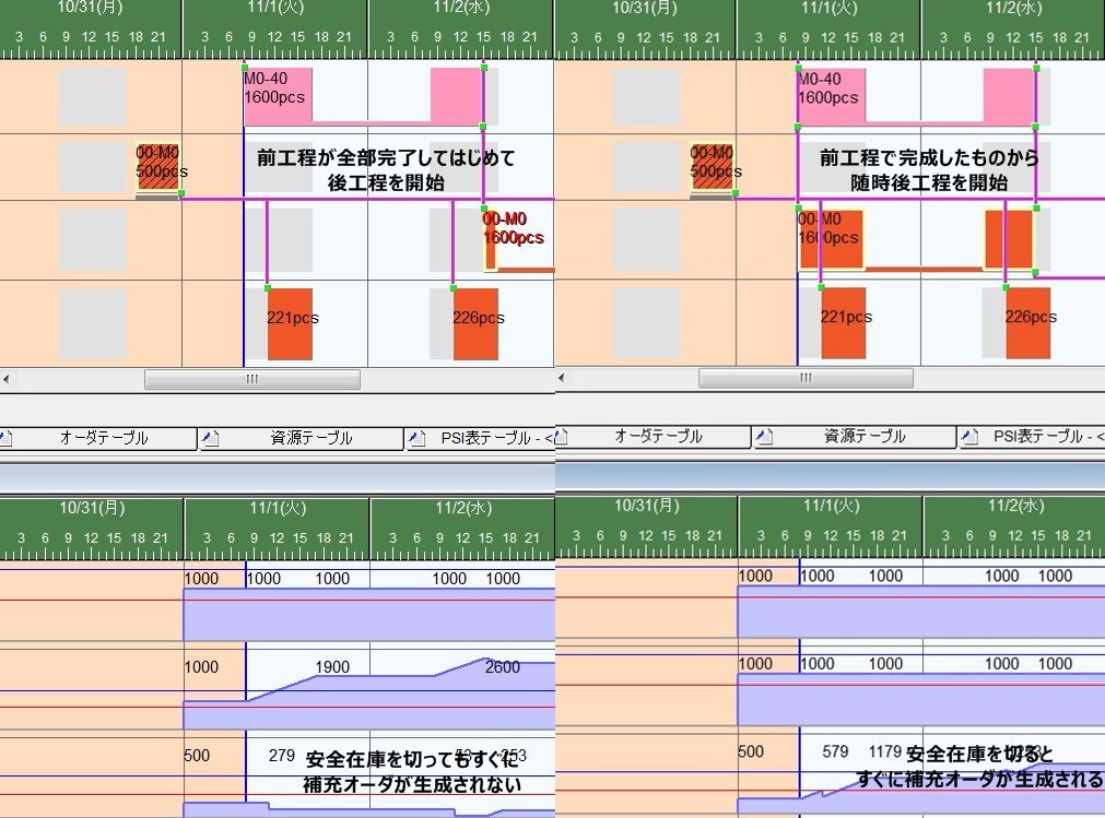
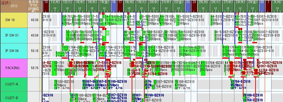
Left: SE, Right: Result of Assigning with SSEE

The aforementioned safety stock is considered during replenishment order generation in order explosion, but the timing of generating replenishment orders varies depending on the inter-process overlap method.
In order explosion, the auto-replenishment function references the manufacturing BOM to fulfill the order list, generating production orders as replenishment orders (children) for shortages in operation input instructions of sales orders, and further generating replenishment orders (grandchildren) for shortages in the input instructions of those replenishment orders.
With an ES (End-Start) overlap method, the current process operation can only start after the preceding process operation is complete, so replenishment orders are generated at the earliest at the start of the current process operation. If shipping or input occurs during the preceding process, there’s a risk of depleting safety stock.
In contrast, with an SSEE (Start-Start End-End) overlap method, the preceding and current processes overlap under the condition that the preceding process doesn’t finish before the current one, allowing replenishment orders to be generated during the preceding process operation, minimizing the risk of depleting safety stock.
However, SSEE assumes a production lot size of one unit, with items flowing individually. In reality, items flow in manufacturing lot or pallet units, so SSEE overlap between processes isn’t always feasible.

Capabilities of the "Leveling" Function

As mentioned, it’s impossible to reflect 100% complete constraints in the scheduler, so the generated schedule’s accuracy isn’t 100%.
However, "leveling" enables the creation of a "theoretically feasible schedule without delivery delays," which MRP’s "stacking" function in a production management system cannot achieve. By setting the inter-process overlap to SSEE, it’s possible to create a schedule that theoretically adheres to safety stock without generating numerous production orders with a lot size of one unit, as in one-piece flow production.

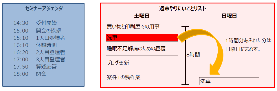
Difference Between Seminar Agenda (Time Axis Occupation) and Weekend To-Do List (Daily Stacking)

When creating an agenda for a seminar, it’s common to assign events to a timeline from start to end time.

This is because assigning tasks to the timeline is critical—e.g., clarifying speaker times so attendees can arrive for their preferred speakers or scheduling a speaker early if they need to catch an evening flight back to Tokyo.
Generally, when creating a schedule, like a Work Breakdown Structure (WBS) in system development projects, tasks are listed on the vertical axis and the timeline on the horizontal axis to clarify when tasks start and end.
In contrast, when imagining a "weekend to-do list" to tackle pending tasks, the focus is on how many tasks can be stacked within the available time over the weekend. Deciding which task to do first can wait until Saturday morning and isn’t a critical planning issue.

Concept of Consuming Maximum Resource Quantity with Required Resource Quantity

When envisioning a "weekend to-do list," there’s an unconscious shift from the typical scheduling mindset of "assigning tasks to a timeline" to "consuming available time with the required time per task."
Abstracting this further, it’s the idea of consuming a "maximum resource quantity" of 8 hours per day with the "required resource quantity" of 2 hours for Project 1, 2 hours for blog updates, 2 hours for a nap, 1 hour for the car wash, and 2 hours for errands.
As another example, in a tunnel furnace heat treatment process, the maximum number of carts that can be set on the belt conveyor per day is 1,000, consumed as "order quantity × required resource quantity of 1 cart."

Since item sizes processed in the tunnel furnace vary, if the inventory of corresponding carts is limited, set the maximum resource quantity of carts to the inventory level. Like the tunnel furnace (main resource) heat treatment time, set the cart transit time to a fixed lead time of 1 day.

Additionally, smaller items allow more units per cart. By setting the mountable quantity in the output instruction per item, one order in the heat treatment process yields output equal to the mountable quantity, meaning the per-unit heat treatment time in the tunnel furnace is inversely proportional to the mountable quantity.